1. papers
- efficient backprop
- Demystifying Deep Convolutional Neural Networks
- He et al., 2015 – he initialization (similar to Xavier)
- adam – https://arxiv.org/pdf/1412.6980.pdf
- alexnet – Krizhevsky et al., 2012. ImageNet classification with deep convolutional neural networks
- residual – He et al, 2015. Deep residual networks for image recognition
- 1×1 conv – Lin et al., 2013. network in network
- inception – Szegedy et al. 2014. Going deeper with convolutions
- conv impl of sliding winds – Sermanet et al., 2014, OverFeat: Integrated recognition, localization and detection using convolutional networks
- yolo – redmon et al. 2015, you only look once: unified real-time object detection
- face rec – taigman et al 2014. DeepFace closing the gap to human level performance
- style transfer – gatys et al., 2015. A neural algorithm of artistic style.
- gru – cho et al., 2014. On the properties of neural machine translation: Encoder-decoder approaches
- gru – chung et al., 2014. Empirical Evaluation of Gated Recurrent Neural Networks on Sequence Modeling
- lstm – hochreiter & schmidhuber 1997. long short-term memory
- embeddings similarities – Mikolov et.al.,2013, Linguistic regularities in continuous space word representations
- learning word embeddings – Bengio et.al.,2003, A neural probabilistic language model
- word2vec – mikolov et.al., 2013 Efficient estimation of word representations in vector space
- GloVe – pennington et.al.,2014. GloVe: Global vectors for word representation
- bias(gender..) – bolukbasi et.al.,2016. Man is to computer programmer as woman is to homemaker? Debiasing word embeddings
- seq-to-seq – cho et.al.2014 Learning phrase representations using RNN encoder-decoder for statistical machine translation
- seq-to-seq – sutskever 2014. Sequence to seq learning with neural networks
2. basics
2.1. Vectorizing and equations (Andrew Ng notation)
         __  a1[1]
        /          \
     x1 _           \_
      \\ \_  a2[1] _  \__
       \\           \__  \
     x2 \\             \__
         \\_ a3[1] ______/ a[2] --- y_hat
         |
     x3  \               /
          \_ a4[1] _____/

       a1[1] = sigmoid(z1[1])
       z1[1] = w1[1]_T*x + b1[1]

    each unit in the layer works as a small logistic regression unit

          -----------
       --/     |     \--
     /         |        \
    /          |         \
    -  w_T*x+b=|sigmoid(z)|
    \     z    |     a   /
     \         |        /
       --\     |     /--
          -------+---
               |activation|

    - n - number of input features
    - m - number of training examples
    - [l] - layer number
    - n[l] - number of units at l layer
    - i - node number in the layer
    - z1[1] - linear output of the 1node from 1layer
    - a1[1] - output of the 1node from 1layer - activation output (thats why 'a')
    - x - input features, column vector [n x 1]
    - X - stacked features of all examples [n x m]
    - b1[1] - single number for a single node
    - w_i[l] - params for each node for each layer [n[l-1] x 1] n[l-1] - number of nodes on previous layer)
    - W[l] - transposed params of each node of single layer stacked into rows
              [ w_1[1]_T ]
              [ w_2[1]_T ]
              [ w_3[1]_T ]
              [ w_4[1]_T ]
        dimension - [n[l] x n[l-1]]
                  [4 x 3]
    - z = w_T * x + b
      Z[l] = W[l] * X + b[l]
      (~+ b~ - broadcasted to each column)
      # dimensions
      Z[l] ~[n[l] x m]~ = W[l] ~[n[l] x n[l-1]]~ * X ~[n[l-1] x m]~ + b[l] ~[n[l] x 1]~
    - y_hat = a = sigmoid(w_T * x + b) = a
      Y_hat = A[l] = sigmoid(Z[l])
    - optimizations for calculation: vector x -> matrix X - by number of examples; w -> matrix W - by number of nodes on this layer
2.1.1. notation(andrew ng)
      Notation:
      Superscript  [l]  denotes a quantity associated with the  lth layer.
      Example:  a[L]  is the  Lth  layer activation.  W[L]  and  b[L]  are the  Lth  layer parameters.
      Superscript  (i)  denotes a quantity associated with the  ith  example.
      Example:  x(i)  is the  ith  training example.
      Lowerscript  i  denotes the  ith  entry of a vector.
      Example:  ai[l]  denotes the  ith  entry of the  lth  layer's activations)
2.1.2. multiple training examples
                <----- different examples --->
               /\
               ||      |       |       |
              diff     |       |       |
      A[1] =  hidden  a[1](1) a[1](2) a[1](3)
              units    |       |       |
               ||      |       |       |
               \/
      Same for Y,Z
      For X - number of features over different examples
2.1.3. activation
- sigmoid - better for output then tanh
- tanh = (e^z - e^-z)/(e^z + e^-z) - better then sigmoid for hidden layers, centers to 0 which is easier for the next layer
- RELU(z) = max(0,z), when 0 derivative can be 1 or 0, not significant
- LeakyRELU - when z < 0 derivative is not 0 but small
You need non-linear activation because otherwise hidden layers doesn't make any difference, the whole computation is linear.
If you have sigma only in the last output layer, then it's not different to logistic regression.
The only case when linear activation makes sense - is when y is real number, e.g. doing regression problem - predicting house price
then it makes sense to use linear activation only in the output layer
[/sourcecode]
</div>
</div>
<div id="outline-container-orgb87e364" class="outline-4">
<h4 id="orgb87e364">derivatives notation</h4>
<div class="outline-text-4" id="text-orgb87e364">
∂J/∂a=da
2.1.4. derivatives
      sigmoid'=g(z)(1 - g(z)) = a(1 - a)
      tanh'=1-(tanh(z))^2
      relu'={0 if z < 0; 1 if z > 0; undefined if z = 0}
2.1.5. backprop
      need to compute derivatives:
      dW[1] := dJ/dW[1],  db[1] = dJ/db[1],  ....
      and then change w/b params:
      W[1] := W[1] - alpha*dW[1]
      ...
      dZ[2]=A[2]-Y
      dW[2]=1/m * dZ[2]*A[1]_T
      db[2]=1/m * np.sum(dZ[2],axis=1,keepdims)    ([n[2],1])
      dZ[1]=W[2].T*dZ[2] *elem-wise-product* g[1]'*z[1]      ([n[1],m] . [n[1],m])
           (or)=dA1 * np.int64(A1 > 0)
      dW[1]=1/m * dZ[1]*X_T
      db[1]=1/m * np.sum(dZ[1],axis=1,keepdims)   ([n[1],1])
2.1.6. cost vs loss
      cost - average loss over training examples
          J(W[1],b[1],W[2],b[2]) = 1/m * Sum[1:m](L(y_hat,y))
      loss function - the one which we optimize
       - CrossEntropy: L(y,a)=−(ylog(a)+(1−y)log(1−a))
         for results [0,1]
       - MAE(L1) - mean absolute error - just sum of abs of diff
       - MSE(L2) - mean sq error - sum of sqrs divided by number
2.1.7. init randomly and not to 0
      because hidden units are symmetric, compute similar function over similar data
      b - can be initialized to 0
      w - rand*0.01 - you want it to be close to the middle (but not always)
2.2. model decision list
- #layers
- #hidunits
- learnrate
- actfuncs
2.3. model implementation flow
- Initialize parameters / Define hyperparameters
- Loop for num_iterations:
a. Forward propagation
b. Compute cost function
c. Backward propagation
d. Update parameters (using parameters, and grads from backprop) - Use trained parameters to predict labels
3. regularization
3.1. bias vs variance
- high bias - underfitting
- high variance - overfitting
  bias - high error
  variance - dev error higher then train
3.2. reduce bias/variance
high bias - bigger net, train longer
high var - more data, regul, net architecture
3.3. reduce bias: regularization l1/l2
- l1 norm: ||w||_1 = |w1|+|w2|+...|wn|
  np.linalg.norm
- l2 norm: ||w||_2 = |w1|^2+|w2|^2+...   (element wise sqr and sum)
  J=1/m * Sum(L(y,y^)) + lambda/2m * ||w||_1(or 2)
  intuition: when lambda is high(higher effect of regularization) - the higher penalty on W produced, making network "simplification" effect
  consider tanh activation - when close to 0 (small z, high regularization) - it is more linear (simpler function)
  dWl = .. + lambda/m * W
  L2-regularization relies on the assumption that a model with small weights is simpler than a model with large weights
3.4. reduce bias: dropout: when on each iteration we drop some of the nodes
Training Phase: For each hidden layer, for each training sample, for each iteration,
ignore (zero out) a random fraction, p, of nodes (and corresponding activations).
drop % from A[1] (A[1] * D[1])
Divide  A[1]  by keep_prob (inverted dropout - result of the cost will still have the same expected value as without drop-out)
Testing Phase: Use all activations, but reduce them by a factor p (to account for the missing activations during training).
3.5. other regularization techniques:
data augmentation techniques - flip images
early stopping - train error lowers but dev set error may grow again (it has local minimum)b
4. optimization
4.1.
x := x - mu
x := x / sigma^2 (variance)
normalizing input features makes learning faster
the function values are distributed uniformly over all dimensions
4.2. ..what is gradient?
gradient - is a col-vector of partial derivatives of the function f[R^n->R]
depicts speed and direction of function increase (or decrease)
4.3. vanishing, exploding gradients, initialization
deeper network is, params get exponentially big or small - each next layer is like multiply w11*w22*....
when values are too big we have very large cost function values, and it will go down very slow
(another intuition) if net is very deep, it is harder for backprop to propagate changes in early layers
need to initialize smart
let's put Var(w)=2/n (variance)
wl=rand()*sqrt(1/n[l-1]) (or 2 for relu - called He, works well for networks with ReLU activations)
for tanh - sqrt(1/n[l-1]) - xavier (for He we have 2/..)
for some other - sqrt(2/(n[l-1]+n[l]))
4.4. gradient checking
basically to check correctness if implement backprop ourselves
TethaVector(w1,b1,w2,b,2....)
dT(dw1,db1....)
for each i:
dTapprox = (J(...Ti+e)...)-J(...Ti-e,...))/2e
dT ~ dTapprox
Check  L2(dT-dTapprox)/(L2(dT) - L2(dTapprox))
for e=10-7, check~10-7  - it's ok
if check 10-5 - suspicious, if less - worry
4.5. batch/stochastic/mini gradient decent
batch - this is just when all examples used - a batch
mini - when you have a lot of examples (5000000) - you can operate in 1000 batches and progress faster
stochastic - when mini-batch is 1 size
4.6. optimizations
Exponentially weighted average: V0=0, Vt=Beta*Vt-1 + (1-Beta)*Theta_t;  Beta=0.9 ~ 10 last values, Beta=0.98 ~ 50 last values
Bias correction:  (fixes beginning of weighted averages)  Vt/(1-Beta^t)  - for higher t will not have impact
4.6.1. grad desc with momentum
4.6.2. RMSprop
4.6.3. Adam optimization
Vdw = Beta1*Vdw + (1-Beta1)*dw
Sdw = Beta2*Sdw + (1-Beta2)*dw^2
V_corrected_dw = Vdw/(1-Beta1^t)
S_corrected_dw = Sdw/(1-Beta2^t)
w := w-alpha * V_corrected_dw / (sqrt(S_corrected_dw) + epsilon)
..
alpha - needs to be tuned
Beta1: 0.9 (usually)
Beta2: 0.999
epsilon: 10^-8
4.6.4. learning rate decay
when approaching optimum, it's better to slow down so we will not miss it
alpha = 1 / (1 + decay_rate * epoch_num) * alpha0
exponential: 0.95^epoch_num * alpha0
another: k/sqrt(epoch_num) * alpha0 or k/sqrt(t)*alpha0
descrete staircase
4.6.5. local optima
rule: 2/3d intuition/observations do not transfer very good to highly-dim space
saddle: if grad=0 - it is convex/concave function in each direction, but chances int 20k-dims space is very small, instead it is much more likely it is saddle
it is unlikely to get stuck in local optima
plateau: when saddle is very wide/long, when derivative is close to zero for a long time
5. tuning & hyperparameters
5.1. hyperparameter tuning
params to tune:
| alpha | first priority |
| Beta ~ 0.9 | second |
| Beta1, Beta2, sigma | forth |
| #layers | third |
| #hidden units | second |
| learning rate decay | third |
| mini-batch size | second |
     simple - grid search (bad)
     better - random because tried variants have less distribution (all except one are always bound to grid values)
     next step - zoom in some region of hyperparameters and sample more densely
5.1.1. use better scale
e.g. for alpha 0.001 to 1 - better to use logarithmic scale
r = -4*np.random.rand() <- [-4,0]
alpha = 10^r <- 10^-4..10^0
r[a,b] <- a=log10(0.001)
for Beta -> (1-Beta)
5.1.2. in practice
- pandas – babysitting (watch each day and adjust learning rate)
- caviar – many models in parallel
5.2. batch normalization
     for each minibatch:
       i - example index
       mu=1/m*Sum(z(i))
       sigma^2=1/m*Sum(z(i)-mu)^2
       z_norm(i)=(z(i)-mu)/sqrt(sigma^2+epsilon)
       z_tilda(i)=gamma*z_norm(i)+Beta
     the same as [[normalization]] but for each layer (not only input)
     makes learning faster, makes weights "deeper" - deeper layers are more robust to changes
     distribution of features on layer L shifts less (less covariate shift)
     in other words, it reduces coupling between layers
     it has slight regularization effect, as it introduces some noise to each layer, but higher mini-batch size reduces this effect
                      ^ z[2]2              ^ z[2]2
                      |                    |
                      o o                 x|x
                    x |o o  z[2]1        x |x   z[2]1
              -----x-x+------->    ------o-+-o----->
                     x| x                 o|o             mean 0     (beta in fact)
                      |                    |              variance 1 (gamma in fact)
                      |                    |
5.2.1. “covariate shift”
      when input data distribution changes, you should retrain even though it is the same function you tried to learn (e.g. trained only on black cats)
      in the neural networks, each layer after first suffers from this problem, as A1,2,3,.. from layer L-1 on layer L are as if the input features for the layer 1
      so the input distribution changes all the time for the layer L
5.2.2. batch norm at test time
      at train you operate in mini-batches, but at test you probably to process 1 at a time
      for that reason you need some estimation for mu/sigma^2 so you can use in test formulas
      one can do exponentially weighted averages over each minibatch for a given layer
      X{1},     X{2},.. (minibatches)
      mu{1}[l], mu{2}[l] ...
      Theta1    Theta2
      sigma...
      z_norm=z-mu / sqrt(sigma^2+epsilon)  z_tilda=gamma*z_norm+Beta
5.3. softmax regression
     e.g. 4 classes
                  layer L
      ( )          ( )
  X-> ( ) => .. => ( ) => y_hat
      ( )          ( )
                   ( )
        *softmax layer* - output layer
      at layer ~l~
      ti = e^(z_i[l])
      a_j[l]=e^(z_j[l])/sum(i=1:4)ti
softmax activation function a[l]=g[l](z[l])
    for example:
    when no hidden layers, just softmax (*softmax regression*) - generalization of logistic regression (linear function) to multiple classes
    vs. hard-max (1 where biggest element in vector, others 0 [1,0,0,0].T)
5.3.1. how to train
Loss function:
y = [0100].T   a[l]=y_hat=[0.3 0.2 0.1 0.4].T  C=4
L(y_hat,y) = -Sum[1:4]y(i)*log(y_hat(i)) = -log(y_hat(2))
if learning trying to make L small -> y_hat(2) as big as possible  (so it works)
Cost:
J(w[l],b[l],..) = 1/m*Sum[i:m]L(y_hat(i),y(i))
Vectorizing:
Y shape (4,m)    Y_hat shape (4,m)
GradDescent:
dz[l]=y_hat-y   (4,1)   ->   =∂J/∂z[l] (it should equal)
6. tensorflow simple example
       import numpy as np
       import tensorflow as tf

       # -----------------------
       # coefficients used for placeholders (input features)
       #coefficients=np.array([[1.],[-10.],[25.]])
       #coefficients=np.array([[1.],[-20.],[100.]])

       # -----------------------
       # define a parameter to be searched
       w = tf.Variable(0,dtype=tf.float32)

       # -----------------------
       # placeholder - something that you provide values for later
       #x = tf.placeholder(tf.float32, [3,1])

       # -----------------------
       # heart of tensorflow program - tf constructs computation graph, and can automatically build backward prop
       cost=tf.add(tf.add(w**2,tf.multiply(-10.,w)),25)
       # or
       # cost=w**2-10*w+25
       # or when input x used
       #cost=x[0][0]*w**2+x[1][0]+x[2][0]

       # -----------------------
       # optimization algorithm
       train=tf.train.GradientDescentOptimizer(0.01).minimize(cost)

       # -----------------------
       # idiomatic tf
       init=tf.global_variables_initializer()
       session=tf.Session()
       session.run(init)
       print(session.run(w))
       # or
       # with tf.Session() as session:
       #     session.run(init)
       #     print(sessions.run(w))
       # 0.0

       # -----------------------
       # running 1 iteration of optimizer
       session.run(train)
       # to supply input values
       # when you do mini-batch grad, then on each iteration you supply different batch using feed_dict
       #session.run(train, feed_dict={x:coefficients})
       print(session.run(w))
       # 0.1

       # -----------------------
       # running 1000 iterations
       for i in range(1000):
           session.run(train)
       print(session.run(w))
       # 4.99999
       # or 9.99998 with coefficients
7. structuring
7.1. orthogonalization
tune in order
1. fit training set well on cost func (~human level perf)
   bigger net, adam
2. fit dev
   regularization, bigger train set
3. fit test
   bigger dev set
4. performs well in real world
   change dev set or cost func
7.2. precision vs recall, single numb eval metric
prec - what % of recognized are actually cats
recall - what % of all are recognized as cats
harmonic mean = 2/(1/p+1/r)
you can pick some other metric - but single is easier to work with
7.3. satisficing vs optimizing
e.g. satis - accuracy, latency - satis
if N metrics - pick 1 as optim, rest N-1 as satis
7.4. train/dev/test
distribution
1. uniform across regions
2. consider future
3. consider important
4. dev/test same distribution

   size
   if a lot data (1000000) train/dev/test 98/1/1%
   test - big enough to be confident in performance (10000,100000)

   when to change dev/test or metrics
   e.g. A vs B, A have better accuracy but has porno images, then B is better for users
   so we can redefine metric including high weight for porno img
   (orthogonalization for this case) 1. define metric for classifier. 2. find out how to do well with this metric

   change dev/test set - e.g. when in real world people suuply blurry etc. - means dev/test does not correspond real world distribution
7.5. vs humans
accuracy vs time - accuracy raises over time but plateau after human level
- human error - the level of humans
- Bayes optimal error - is the top  your alg can reach, not far from human error
- if worse than humans: 1. get labels from hum 2. manual analysis 3. better bias/var analysis

  avoidable bias - diff between human and dev/train error
  if human 1%, dev/train 8/10 - reduce bias (7% avoidable bias)
  if human 7.5% - reduce var (10-8)  (0.5% avoidable bias, 2% variance)
  human error ~ Bayes error for a lot of tasks (CV,..)

  surpassing human
  - for structured data cases much better: - online ad - product recommend - logistics - loan approval
  - for some natural perception as well already: - speech recognition - some image recognition - medical
7.6. dev/test/train & bias/var
     human-level
        ~/\~
        ~||~  avoidable bias: bigger net, train longer, better optimization alg (momentum, rmsprop, adam), better net architecture(rnn/cnn), hyperparameter search
        ~\/~
     training error
        ~/\~
        ~||~  avoidable var: regularization(l2, dropout, data augmentation), getting more data, net architecture, hyperplane search
        ~\/~
     train-dev error
        ~/\~
        ~||~  data mismatch
        ~\/~
     dev error
            degree of overfitting to dev set
     test error
7.7. error analysis
fix incorrect labels only if that is worthwhile - measure % of those, impact
same process for dev/test - make sure sam distribution
train can be slightly different distribution
go and manually check examples
7.8. train/dev/test mismatch
interesting insight:
if you have desktop and mobile(low quality) pictures
its better to train on desktop and use mobile for dev/test - gives better results

better in another case (quite similar) - speech recognition in car (rear mirror)
it's better to combine varios sources to train on (smart speaker, voice keyboard, car rear view, etc)

# bias and var
sometimes, when we have different datasets in train/dev it makes sense to pick some part of train test as dev to do a test and make sure e.g. the problem is with variance (and not with data mismatch)
7.8.1. how to address data mismatch?
1. manually analyse difference
2. try to match - artificial synthesis e.g. add car noise (background noise)
   but beware of overfitiing - if 1hour of noise net will overfit to it
8. multiple-tasks learning
8.1. transfer learning
it makes sense when
- task A and B have same input x
- you have a lot of data for the problem you're transferring from and less data for the problem you're transferring to
  e.g. 10mil img recognition -> 1000 radiology diagnosis
  speech rec 10000hours -> 1h wakeword
- features from A can be valuable to B

  pre-training - when re-train all net with previous layers as well
  fine-tuning - when you keep previous layers and retrain only last
8.2. multi-task learning
like soft-max but can have multiple labels - e.g. self-driving recognition - one image, car|pedestrian|stop|trafficlight output labels
makes sense when
- benefit from sharing low-level features
- quite similar amount of data for each task
- can train big enough net to do well on all tasks
  used rarely, transfer is used much more
8.3. end-to-end learning
traditional speech recognition
audio -mfcc-> features -ml-> phonemes words -> transcript
works if you have ~3000hours
direct net from audio to transcript works better when > 10000h/100000h

Pro:
• Let the data speak
- By having a pure machine learning approach, the neural network will learn from x to y. It will
  be able to find which statistics are in the data, rather than being forced to reflect human
  preconceptions.
  • Less hand-designing of components needed
  - It simplifies the design work flow.
    Cons:
    • Large amount of labeled data
    - It cannot be used for every problem as it needs a lot of labeled data.
      • Excludes potentially useful hand-designed component
      - Data and any hand-design’s components or features are the 2 main sources of knowledge for a
      learning algorithm. If the data set is small than a hand-design system is a way to give manual
      knowledge into the algorithm.
9. advanced
9.1. common architectures
https://data-notes.co/a-gentle-introduction-to-neural-networks-for-machine-learning-d5f3f8987786
- perceptron
- cnn
- rnn
- lstm
- gru
- hopfield
- boltzmann
- deep belief
- autoencoders
- gan
10. cnn
10.1. notation
- Superscript $[l]$ denotes an object of the $l^{th}$ layer.
  - Example: $a^{[4]}$ is the $4^{th}$ layer activation. $W^{[5]}$ and $b^{[5]}$ are the $5^{th}$ layer parameters.

- Superscript $(i)$ denotes an object from the $i^{th}$ example.
    - Example: $x^{(i)}$ is the $i^{th}$ training example input.

- Subscript $i$ denotes the $i^{th}$ entry of a vector.
    - Example: $a^{[l]}_i$ denotes the $i^{th}$ entry of the activations in layer $l$, assuming this is a fully connected (FC) layer.

- $n_H$, $n_W$ and $n_C$ denote respectively the height, width and number of channels of a given layer. If you want to reference a specific layer $l$, you can also write $n_H^{[l]}$, $n_W^{[l]}$, $n_C^{[l]}$.
- $n_{H_{prev}}$, $n_{W_{prev}}$ and $n_{C_{prev}}$ denote respectively the height, width and number of channels of the previous layer. If referencing a specific layer $l$, this could also be denoted $n_H^{[l-1]}$, $n_W^{[l-1]}$, $n_C^{[l-1]}$.
10.2. edge detection
– convolution operator
       6x6 grey scale image
     +-----+-----+-----+-----+-----+-----+
     | *3* | *0* | *1* |  2  |  7  |  4  |      3x3 filter          4x4 output
     +-----+-----+-----+-----+-----+-----+       (kernel)        +-------+-----+-----+-------+
     | *1* | *5* | *8* |  9  |  3  |  1  |     +---+---+---+     |  *-5* |  -4 |   0 |   8   |
     +-----+-----+-----+-----+-----+-----+     | 1 | 0 |-1 |     +-------+-----+-----+-------+
     | *2* | *7* | *2* |  5  |  1  |  3  |     +---+---+---+     |  -10  |  -2 |   2 |   3   |
     +-----+-----+-----+-----+-----+-----+  *  | 1 | 0 |-1 |  =  +-------+-----+-----+-------+
     |  0  |  1  |  3  | =1= | =7= | =8= |     +---+---+---+     |   0   |  -2 |  -4 |  -7   |
     +-----+-----+-----+-----+-----+-----+     | 1 | 0 |-1 |     +-------+-----+-----+-------+
     |  4  |  2  |  1  | =6= | =2= | =8= |     +---+---+---+     |  -3   |  -2 |  -3 | =-16= |
     +-----+-----+-----+-----+-----+-----+                       +-------+-----+-----+-------+
     |  2  |  4  |  5  | =2= | =3= | =9= |
     +-----+-----+-----+-----+-----+-----+

     element-wise
     3x1 + 1x1 + 2x1 + 0x0 + 5x0 + 7x0 + 1x-1 + 8x-1 + 2x-1 = -5
     ...

     tf: tf.nn.conv2d

     keras: Conv2d

     *takeaway*:
     vertical edge - is the 3x3 region where is bright pixels on the left and dark pixels on the right (the middle is not significant)

     *takeaway2*:
     instead of 1/0/-1 in the filter - we can treat those as parameters of the model to learn (big improvement)
10.2.1. simple example (grey image)
     +----+----+----+---+---+---+
     | 10 | 10 | 10 | 0 | 0 | 0 |
     +----+----+----+---+---+---+                       +-----+----+----+-----+
     | 10 | 10 | 10 | 0 | 0 | 0 |     +---+---+---+     |  0  | 30 | 30 |  0  |
     +----+----+----+---+---+---+     | 1 | 0 |-1 |     +-----+----+----+-----+
     | 10 | 10 | 10 | 0 | 0 | 0 |     +---+---+---+     |  0  | 30 | 30 |  0  |
     +----+----+----+---+---+---+  *  | 1 | 0 |-1 |  =  +-----+----+----+-----+
     | 10 | 10 | 10 | 0 | 0 | 0 |     +---+---+---+     |  0  | 30 | 30 |  0  |
     +----+----+----+---+---+---+     | 1 | 0 |-1 |     +-----+----+----+-----+
     | 10 | 10 | 10 | 0 | 0 | 0 |     +---+---+---+     |  0  | 30 | 30 |  0  |
     +----+----+----+---+---+---+                       +-----+----+----+-----+
     | 10 | 10 | 10 | 0 | 0 | 0 |
     +----+----+----+---+---+---+

          |--+--+-+-+-+--|       |----------------|     |---------------------|
          |       |      |       |     |    |     |     |    |     |     |    |
          | white | grey |   *   |white|grey|black|  =  |grey|white|white|grey|
          |       |      |       |     |    |     |     |    |     |     |    |
          |-------+------|       |-----+----+-----|     |----+-----+-----+----|
white vertical stripe – we detected strong vertical edge (thick because very small dimensions)
10.2.2. more examples
      - flip colors
        darker on the left, brighter on the right - results in |grey|black|black|grey|  (|0|-30|-30|0|)
        you can take absolute
      - horizontal (10 and 0)
        10 10 10  0  0  0
        10 10 10  0  0  0     1 1 1        0   0   0   0
        10 10 10  0  0  0  *  0 0 0        30 10 -10 -30
        0  0  0  10 10 10    -1-1-1        30 10 -10 -30
        0  0  0  10 10 10                  0   0   0   0
        0  0  0  10 10 10
        this artifact in the output comes from this transition region - this is unnoticable on large scale
      - 3x3 - is only one of the ways, could be:
        1 0 -1      3  0 -3
        2 0 -2  or  10 0 -10
        1 0 -1      3  0 -3
        Sobel       Scharr
Sobel – put a little bit more weight to middle pixels
we could learn this filter weights as parameters of the model! instead of putting by hand
it could then learn 45/70 degrees etc, or maybe end up with Sobel filter etc.
10.3. padding
     n-input
     f-filter (usually odd)
     p-pad
     padding - adding 1(or more) pixel to the borders (everywhere, 6x6 becomes 8x8)
     two problems:
      - shrinking of image (n-f+1  -   6-3+1 = 4x4 matrix)   a lot in deep network
      - throwing away edges  -  1:1 pixel gets only one convolution
     two types of padding
      - valid convolution (no padding)
      - same (input=output) - p=(f-1)/2
10.4. strided convolutions
     stride = step of moving filter through input (vertically/horizontally), but keep filter entirely within input (no out of edge)
     p-padding 0, s-stride 2
     nxn (7x7) * fxf (3x3)
     then
     (n+2p-f)/s + 1  x  (n+2p-f)/s+1
     3 x 3
10.5. notation: cross-correlation vs convolution
     in strict math what we do here called cross-correlation
     convolution would require flipping filter matrix vertically and horizontally (first row is last and reversed)
     but dl papers started using convolution word

     in signal processing convolution has associativity property (which is not significant in deep learning):
     (A*B)*C=A*(B*C)
10.6. rgb
     filter -> 3x3x3 (3 number of channels)
     6x6x3 * filter  =>  but results in 4x4x1  (no 3)
     single convolution: cube x cube => single output number
10.7. multiple filters (convolution over volume)
     2 filters
      - vertical filter
      - horizontal filter
     results in 4x4x2
     so you can detect multiple features (edges) - e.g. 10 or 128..
     2 - depth of the 3D volume or number of channels
     volume - because rectangle becomes cube
10.8. one layer of ConvNet
     input * filter1 -> Relu(4x4 + b1) -> 4x4
     input * filter2 -> Relu(4x4 + b2) -> 4x4
        => 4x4x2 (a[1])
     in other words this 4x4 is a w[1]*a[0] in this network

     *number of parameters*:
     if 10 filters that are 3x3x3: (27 + 1 (bias)) * 10 = 280 parameters

     *notice*:
     number of parameters doesn't depend on size of image (even 64k x 64k) - still 280
     ->cnn less prone to overfitting - once you learned 280 features you can apply them to any size image

     *notation*:
     for layer l
     hyperparameters: f[l] p[l] s[l] n_c[l] (filter size, padding, stride, number of filters)
     input: n_h[l-1]x n_w[l-1]x n_c[l-1]
     output: n_h[l]x n_w[l]x n_c[l]
     n_hw[l]=(n_hw[l-1]+2p[l]-f[l])/s[l] + 1)
     each filter is: f[l]xf[l]x[n_c[l-1]]
     activations: a[l]->n_h[l]x n_w[l]x n_c[l]
       A[l]: m x n_h[l] x n_w[l] x n_c[l]
     weights: f[l]x f[l]x n_c[l-1]x n_c[l]
     bias: n_c[l] - (1,1,1,n_c[l])

     $$ n_H = \lfloor \frac{n_{H_{prev}} - f + 2 \times pad}{stride} \rfloor +1 $$
     $$ n_W = \lfloor \frac{n_{W_{prev}} - f + 2 \times pad}{stride} \rfloor +1 $$
     $$ n_C = \text{number of filters used in the convolution}$$


     *notice*:
     depth of the filter should equal to depth of input layer
     and number of filter will determine depth of output layer
10.9. simple ConvNet
     input:
       39x39x3
       n_h[0]=n_w[0]=39
       n_c[0]=3
     layer1:
       f[1]=3
       s[1]=1
       p[1]=0
       10 filters
       first layer output: 37x37x10
       n_c[1]=10
     layer2:
       f[2]=5
       s[2]=2
       p[2]=0
       20 filters
       17x17x20                `    /---/`
     layer3:                   `   /   /|`
       f[3]=5                  `  /   / |`
       s[2]=2                  ` /   /  /`
       p[2]=0                  `/---/  / `
       40 filters              `|   | /  `
       7x7x40                  `|   |/   `
       computed 40 features    `/---/    `
       usually we can flatten this out in vector (size 1960)
     and pipe through logistic/softmax output

     in general the dimensionality of each layer will slowly reduce through network
10.10. type of layers
      - Convolution (Conv)
      - Pooling (POOL)
        instead of element-wise multiply - just pick max number.  usually no padding
        when f=2, s=2, no weights to learn - keep only max number out of 4 (the most important feature?)
        no parameters, no backward propagation, nothing to learn
        It helps reduce computation, as well as helps make feature detectors more invariant to its position in the input.
        $$ n_H = \lfloor \frac{n_{H_{prev}} - f}{stride} \rfloor +1 $$
        $$ n_W = \lfloor \frac{n_{W_{prev}} - f}{stride} \rfloor +1 $$
        $$ n_C = n_{C_{prev}}$$
        !! it acts on each volume layer (channel) separately, doesn't change number of channels
        - average pooling: take avg instead of max (rarely used)
      - Fully connected (FC)
        like a normal NN layer - all nodes are connected fully
10.11. LeNet-5
     digit recognition
     32x32x3 --f=5,s=1--> Conv1[28x28x6] --maxpool[f=2,s=2]--> POOL1[14x14x6] --f=5,s=1-->
       --> Conv2[10x10x16] --maxpool[f=2,s=2]--> POOL2[5x5x16] --> flatten[400x1] -->
       --> FC3[120x1] --> FC4[84x1] -> softmax[10 outputs]
     w[3] (120,400) b[3] 120
     h/w decrease, number of channels increase
| activation shape | activation size | # parameters | |
|---|---|---|---|
| Input: | (32,32,3) | 3072 | 0 |
| CONV1(f=5,s=1) | (28,28,8) | 6272 | 608 |
| POOL1 | (14,14,8) | 1568 | 0 |
| CONV2(f=5,s=1) | (10,10,16) | 1600 | 3216 |
| POOL2 | (5,5,16) | 400 | 0 |
| FC3 | (120,1) | 120 | 48120 |
| FC4 | (84,1) | 84 | 10164 |
| Softmax | (10,1) | 10 | 850 |
10.12. advantages of cnn
     - parameter sharing
       a feature detector (filter) that is useful in one place is probably useful in another part
       e.g. learned vertical edges are useful in a lot of places (as well higher features (cat in different parts of image))
     - sparsity of connections
       in each layer each ouput depends only on small subset of input (convolued filtered inputs)
     - translation invariance
       less prone to shifting objects on the image
10.13. classic networks
     - LeNet-5
     - AlexNet
       [227x227x3] --conv[f=11,s=4]--> [55x55x96] --maxpool[f=3,s=2]--> [27x27x96]
         --conv[f=5,same]--> [27x27x256] --maxpool[f=3,s=2]--> [13x13x256]
         --conv[f=3,same]--> [13x13x384] --conv[f=3,same]--> [13x13x384]
         --conv[f=3,same]--> [13x13x256] --maxpool[f=3,s=2]--> [13x13x256]
         --maxpool[f=3,s=2]--> [6x6x256] --flat--> [9216] --fc--> [4096]
         --fc--> [4096] --softmax[1000]
       ~60m params to train
       using ReLU

     - VGG-16
       always same filters and same pooling: CONV=f=3x3,s=1,same    MAX-POOL=2x2,s=2
       [224x224x3] --2xCONV64--> [224x224x64] --POOL--> [112x112x64] --2xCONV128--> [112x112x128]
         --POOL--> [56x56x128] --3xCONV256--> [56x56x256] --POOL--> [28x28x256] --3xCONV512--> [28x28x512]
         --POOL--> [14x14x512] --3xCONV512--> [14x14x512] --POOL--> [7x7x512] --FC--> [4096]
         --FC--> [4096] --softmax--> [1000]
       ~138m params - pretty big
       VGG-19
10.14. ResNet
residual block:
     regular path from a[l] to a[l+2]:
     a[l] -o-> Linear -> ReLU -a[l+1]-> Linear -x-> ReLU -> a[l+2]
           \                                    /
            \___shortcut from a[l] to a[l+2]___/

     a[l+2]=g(z[l+2] + *a[l]*)
     (one more name - skip connection)
residual network is a network of residual blocks
     training err
     ^
     |
   ~ |        in regular nn error goes up again after increase to some number of layers
   ~ |        in resnet it keeps going down - helps training very deep nets
     |
     |
     ------------------>
              #layers
why it works (intuition):
a[l+2]=g(w[l+2]a[l+1] + b[l+2] + a[l])
if you apply weight decay or l2 regularization it will shrink w[l+2] and b[l+2]
this may mean a[l+2] ~ a[l] - it's easy to learn identity function
adding residual network at least doesn't hurt performance
on the contrary in very deep nets - some layers start to hurt performance, while in resnet - it may improve but not hurt

one note: dimension of start of block and end block should be equal, otherwise you may apply Ws matrix to a[l] vector (multiply to match a[l+2] dimension)
ResNet are quit deep <no image here>
10.15. 1×1 convolutions
the depth matters - it is like cube with 1x1 face
each filter will take a single "tube" from input, multiply, apply ReLU and output one number
single filter - is is like fully connected single-node layer of classical net
if there are multiple filters - then its like fully connected multi-node layer
thats why it is called network in network

something we can do with this:

[28x28x192] --32xCONV1x1--> [28x28x32]
to shrink H/W - can use Pooling layer
but if you want shrink number of channels - can use Conv1x1

*you can control number of channels*
10.16. inception network
we need to go deeper (Nolan, Inception)
     conv or pool? lets do them all

     [28x28x192] --1x1-> [28x28x64]
                 \__3x3,same__> [28x28x128]
                  \__5x5,same__> [28x28x32]
                   \__MAX_POOL__> [28x28x32]
                stack all of this into [28x28x256]
       one problem - for layer 5x5 you need to do ~120M multiplications
       solution - do the 16xCONV1x1 -> [28x28x16] --32xCONV5x5--> [28x28x32]
       in the middle - "bottleneck layer"
       ~12.4M multiplications
       ??does it hurt accuracy??

     inception module:

                                   -> 64xCONV1x1
                    96xCONV1x1     ->128xCONV3x3
     [28x28x192] -> 96xCONV1x1     -> 32xCONV5x5 -> concat
                    192xMAXPOOL3x3 -> 32xCONV1x1

     network - puts together a lot of such modules
note: some layers in inception network can have softmax outputs (kind of early outputs) – this has regularization effect
     -----------big-network------output
        \____output
10.17. transfer learning
e.g. you want to recognize which one of your 3 cats
- download opensource net with trained weights (e.g. output 1000 classes)
- remove final softmax, replace with softmax with your 3 cats classes
- to speed up you can pre-compute (materialize) the all previous layer into one function (save to disk)
- if you have big dataset, you can freeze less layers, and more your layers
- or if you have huge amount of data, you can relearn from scratch
almost always do transfer learning
10.18. data augmentation
we still don’t have enough data
- mirroring
- random cropping
- rotation
- shearing
- local warping
- color shifting
implementing
- separate cpu thread loads and augments image
- separate thread does learning
10.19. tips on winning competitions / benchmarks
- ensembling – train several nets, average outputs (3-15 nets)
- multi-crop at test time – run classifier on multiple versions of test images and average results
11. object detection
classification vs localization vs detection
11.1. localization
     add to final softmax bounding box coordinates
     for 4 classes
     target label y:
       Pc - is there any obj? (if no obj 0, and rest are '?')
       bx
       by
       bh
       bw
       c1
       c2
       c3
     Loss:
       - if y1 = 1, squared error of diffs y_hat-y
       - if y1=0, then only squared y_hat1-y_hat
11.2. landmark detection
     e.g. eyes - l1x l1y, l2x l2y - where are edges of eyes
     output vector:
       face?
       l1x
       l1y
       ..
11.3. object detection
     in car detection:
     simple way:
     sliding windows - shift small window of image and check every region (classify)
         then resize window, the resize again
         there should be window with car
     huge disadvantage - huge computation cost

     smarter way - convolutional implementation of sliding windows:
     we could take FC layer in net and turn it into convolution:
     e.g. we had 5x5x16 -> FC[400]:
     5x5x16 --> 400xCONV5x5 --> [1x1x400]
     this last is like fully connected layer
     then, 400xCONV1x1, then 4xCONV1x1 (instead of softmax(4))
     the trick is to have this layers more then 1x1 dimensions
     if imagine running a window on the left upper part of image, this will appear as a left-upper part of final convoluted matrix
     e.g. window 14, stride 2, input 28x28x3 --...-> 8x8x4    - the upper-left 14x14 will appear in upper left in output
11.4. bounding boxes predictions
finding perfect match for box – YOLO (you only look once)
- put 3×3 grid on image (various sizes)
- run localization for each cell – y=[Pc,bx,by,bh,bw,c1,c2,c3].T
- target output 3x3x8
- the idea (probably) is to slice grid so there is only one object in the cell
TODO – yolo is not clear
11.5. intersection over union
     evaluate object localization
     compute size of intersection of predicted and actual box and divide by union of that
     ideally = 1
     "correct" if IoU >= 0.5
     the measure of overlap between 2 boxes
11.6. non-max supression
make sure that algorithm detects each object only once
in yolo, you can get multiple boxes (while having a lot of cells)
- find box with highest prob
- remove those that have not enough IoU (e.g. <= 0.6)
11.7. anchor boxes
     by default each box detects single object, but what if we want multiple?
     what you can do, instead of default *y* output, you stack each anchor object in *y*
     [Pc1,bx,by...,Pc2,bx2,by2,....].T
     previously: each object in training image is assigned to grid cell that contains that object's midpoint
     with two anchor boxes: each object in training image is assigned to grid cell that contains object's midpoint and achor box for the grid cell with highest IoU
     3x3x8 -> 3x3x16
     (probably)for now this algorithm handle fixed number of objects in the cell at the same time e.g. 2 in this example
11.8. YOLO
e.g. 3 classes 1-pedestrian, 2-car, 3-motorcycle
y is 3x3x2x8 (3×3 grid, 2 achors, 8=5+#classes – y output dimension) (in yolo 19×19 grid used)
- to construct training set, you go through each of 9 cells and create vector y
e.g. for empty box y=[0??????..0??????..].T - (non-max supr) get rid of low prob predictions
- (non-max supr) for each class use non-max-suppression to generate final prediction
11.9. r-cnn
     region proposals
     select a few regions (filter out empty) - run some non-dnn algorithm for segmentation (based on gamma/rgb probably)
     r-cnn
     1. propose regions
     2. classify proposed regions
     3. output label + boudning box
     fast r-cnn
     1. propose regions
     2. use conv impl of sliding windows to classify all the proposed regions
     faster
     1. use convolutional net to propose regions
12. face recognition
verification vs recognition(much harder)
12.1. one-shot learning
when the data is small, or when you need to recognize a new face its not a good idea to have long y with all persons classes, better
learning a "similarity" function
d(img1,img2) = degree of diff
if (d <= theta) ...
[/sourcecode]
</div>
</div>
<div id="outline-container-orgb3bdd83" class="outline-3">
<h3 id="orgb3bdd83">siamese network</h3>
<div class="outline-text-3" id="text-orgb3bdd83">
the idea of running 2 identical convnets on 2 different images and then comparing them (theirs encodings) and updating params to learn function d (minimize encoding dist for same person)
having 128 FC output layer
d(x1,x2)=||f(x1)-f(x2)||^2_2 (L2??)
if xi=xj learn params so that L2 is small
otherwise if its different - learn so L2 is large
12.2. triplet loss
positive case and negative case (same person and diff persons (but keep one photo of person1))
anchor/positive anchor/negative
look at 3 at a time
want L2(f(A)-f(P)) - L2(f(A)-f(N)) + alpha <= 0 (L2??)
Triplet function: given 3 images A,P,N
L(A,P,N)=max((f(A)-f(P))^2 - (f(A)-f(N))^2 + alpha, 0)
J=Sum(Li)
training 10k pictures of 1k pictures
How to choose these triplets?
if random - d(A,P)+alpha<=d(A,N) is easily satisfied
choose "hard" d(A,P)+alpha<=d(A,N)
[/sourcecode]
</div>
</div>
<div id="outline-container-org82ec5e9" class="outline-3">
<h3 id="org82ec5e9">learning similarity func</h3>
<div class="outline-text-3" id="text-org82ec5e9">
you could do logistic regression with f(xi)k-f(xj)k as x (wix + b):
y_hat=sigma(Sumk=1:128(wk|f(xi)k-f(xj)k|+b))
the you can do face verification
13. neural style transfer
13.1. what are deep ConvNets learning?
from small edges to more complex patterns
13.2. cost function
G - generated image
C - content image
S - to transfer style from
J(G) = alpha*Jcontent(C,G) + beta*Jstyle(S,G)
1. Initiate G randomly G:100x100x3
2. Use gradient descent to minimize J(G)
3. you actually update image pixels
G = G - alpha/2G * J(G)
content cost function
Jcontent(C,G) - let say you use l layer to compute content cost (it should be not too shallow, not too deep - middle of net)
use pre-trained ConvNet (e.g. VGG net)
Let a[l](C) and a[l](G) be the activation of layer l on the images
if a[l](C) and a[l](G) are similar, both images have similar content
Jcontent(C,G)=1/2*L2(a[l](C)-a[l](G))
style cost function
say you are using layer l's activation to measure "style".
Define style as correlation between activations across channels
(why this captures style? - should look through layers and what they capture - some later layers will capture texture)
correlation - how often that type of textures occurs = how close the style is
k - is channel number
a^[l]_i,j,k = activation at (i,j,k). G^[l] is n_c^[l] x n_c^[l]
Gkk′[l](S) = ∑i=1:nH ∑j=1:nW ai,j,k[l](S) ai,j,k′[l](S)
Gkk′[l](G) = ∑i=1:nH ∑j=1:nW ai,j,k[l](G) ai,j,k′[l](G)
J_style^[l]=1/(2nwnhnc)^2*SumkSumk'(L2(G_S − G_G)) (frobinius form computed on two matrices(images) ||GS-GG||^2_F)
J_style^[l](S,G)=1/(2n_H^[l] n_W^[l] n_C^[l])^2 ∑k∑k′(G_kk′^[l](S) − Gkk′^[l](G))^2
capturing multiple layers
J_style(S,G)=Sum_l(lambda^[l]*J_style^[l](S,G))
overall
J(G) = alpha*Jcontent(C,G) + beta*Jstyle(S,G)
use grad descent (or more sophisticated) that tries to minimize this J
14. 1d and 3d
    the same way as you do convolutions in 2d you can do on 1d
    e.g. electrocardiogram - timeseries you can convolute patterns (e.g 5 filter like 5x5 filter)
    3d - simply additional dimension 14x14x14x16 (16-number of filters)
15. rnn
examples:
- speech recognition
- music generation
- sentiment classification
- dna sequence analysis (AGCCCCTGTGGGA)
- machine translation
- video activity recognition
- name entity recognition
15.1. notation
     x:  Harry Potter and Hermione Grandger invented a new spell
          x^<1> x^<2> x^<3> x^<4> ...........              x^<9>
     Tx=9
     y:
           1     1      0    1         1       0     0  0   0
     Ty=9

     (_^<i> = _<i> here and on)

     when multiple examples:
     x(i)<t>   Tx(i)=9
     y(i)<t>   Ty(i)

     How to represent words in the sentence?
     need a vocabulary (10000 size, but can be much higher these days)
     a        1
     aaron    2
     ..
     and      367
     ..
     harry    4075
     ..
     potter   6830
     ..
     zulu     10000

     Then (using OneHot vector):
     x<1> = [000..010...0].T (1 at 4075)
     each x<t> - is one-hot vector

     so, using this representation and some sequence model we learn a mapping from x -> y
15.2. rnn model
standard network for x<i>->y<i> would not work because:
- inputs, outputs can be different lengths in different examples
- doesn’t share features learned across different positions of text ci
basic block (Tx=Ty)
when making a prediction for y_hat<3> – it gets information not only from x<3> but from x<1> and x<2> as well
15.3. why weights are shared between rnn-cells?
seems like there is no good answer besides less computation
seems like it might be fine for capturing sequential-deps between batches, sentences
15.4. dimension of hidden state (a)
essentially it is a hyperparameter
(from stackoverflow) 50 underfits, 400 overfits
15.5. forwardprop
     a<0> = vector(0)
     a<1> = g(w_aa*a<0> + w_ax*x<1> + b_a)  <- tanh/relu
     y_hat<1> = g(w_ya*a<1> + b_y)  <- sigmoid
     ..
     a<t> = g(w_aa*a<t-1> + w_ax*x<t> + b_a)
     y_hat<t> = g(w_ya*a<t> + b_y)

     lets simplify this notation:
     a<t> = g(w_aa*a<t-1> + w_ax*x<t> + b_a)
     into
     a<t> = g(w_a[a<t-1>,x<t>] + b_a)
     [w_aa;w_ax]=w_a - stack (actually append horizontally)
     if w_aa[100:100], w_ax[100:10000] then w_a[100:10100]
     [a<t-1>,x<t>] = [ a<t-1> ] 100      |   column vector of height 10100
                     [  x<t>  ] 10000    |
     so:
     y_hat<t> = g(w_y*a<t> + b_y)
15.6. backprop
element-wise loss (for a certain word in a sequence):
L<t>(y_hat<t>,y<t>) = -y<t> * log(y_hat<t>) - (1-y<t>) * log(1-y_hat<t>)
overall loss (just sum):
L(y_hat,y) = Sum(t=1:Ty)(L<t>(y_hat<t>,y<t>))
backpropagation through time – the most significant operation (a<t> <- a<t+1> )
15.7. types of networks
- Many-to-many Tx=Ty - e.g. for entity recognition
- Many-to-one
  x=text(nothing to like in this movie), y=0/1 or 1..5 - Sentiment classification
  (same model but no y_hat<1/2/3..> just last y_hat)
- One-to-one (standard neural net (why?))
- One-to-many, x - empty or genre of music  - music generation
  the same as first, but no x<2,3,4,5...> just first x, and each y_hat<i> is supplied into the next a<i+1> as x
- Many-to-many when Tx=/=Ty  - machine translation
  first half of net has no y_hat (encoder), second half has no x<i> (decoder)
- attention based architecture
15.8. language model
The apple and [pair|pear] salad (3.2x10^-13 | 5.7x10^-10)
language model – what is the prob P(sentence) that it will appear now? (like out of all possible sentences)
     Language model estimates the probability of that particular sequence of words
     P(y<1>,y<2>,..y<Ty>)
     fundamental for speech rec as well as translation systems
     To train such a model you need *training set* - a large corpus of english text.
     as well as vocabulary (e.g. 10000)
     Then - *tokenize* ( =>
     /Cats average 15 hours of sleep a day.<EOS>/ (you can use EOS)
     (y<1>,... y<9>), period(,) can be token)
     If unknown word (not in 10000 vocab) (The Egyptian Mau<UNK> is a bread of cat.<EOS>)
Then – model:
What it can do – given previous words, learns to predict next words in the sentence.
Cost function:
     L(y_hat<t>,y<t>) = - Sum(yi<t>*log(y_hat_i<t>))  <-  *softmax loss function*
     L = Sum(L<t>(y_hat<t>, y<t>)))
     Given a new sentence - it can predict what is the probability of this exact sentence
     e.g. 3 words sentence:
     P(y<1>,y<2>,y<3>)=P(y<1>)*P(y<2>|y<1>)*P(y<2>|y<1>,y<2>)
15.9. sampling novel sequences
After you train a sequence model, one of the ways you can informally get a sense of what is learned is to have a sample novel sequences.
Lets say you trained model
now you can do sampling
     you take 1 softmax output y_hat<1> - it is a vector of probabilities (distribution)
     you can use np.random.choice
     e.g. first word was sampled "The", you supply it into second timestamp t=2
     How do you know when sequence ends?
      - until EOS
      - or just fixed e.g. 20
     you can make sure that it doesn't generate UNK word
     this is how you can generate random sentence from learned rnn *language* model
15.10. character-level language model
     vocab=[a,b,c,...0..9,A,..Z]
     is able to handle UNK (Mau - assign a non zero prob)
     requires much more computation, bad at handling longer
15.11. vanishing gradients with rnn
The *cat*, which ....., *was* full
The *cats*, ........ , *were* full
harder to capture this long-term dependencies (layer-early)
if net is very deep, it is harder for backprop to propagate changes in early layers
weakness - the basic rnn has many *local influences*
*vanishing* grads is bigger problem than *exploding* grads with rnns

to fix *exploding* grads - apply *clipping*, just put threshold (np.clip)

in convnets (see residual blocks) loss may increase if net becomes very deep
the same in rnn - if it processes sequence of length 10000 it is basically 10k layer net
15.12. gru (gated recurrent unit)
     gru - modification to rnn hidden layer

     a<t> = g(Wa[a<t-1>,x<t>]+b_a)

     GRU (simplified)
     as we read sentence from left to right we introduce memory cell
     C = memory cell
     C<t> = a<t> (for now, in lstm it is different values)
     at every t, we may rewrite C
     candidate to replace C<t>:
   ->C_tilda<t> = tanh(Wc + b_c)
     Important idea of GRU - Gate:
   ->Γ_u = sigmoid(w_u[C<t-1>,x<t>] + b_u)       (value between 0 and 1, but to develop intuition can think of always 0 or 1)
     _u - stands for update, g - gate
     it decides if replace candidate (may keep or may substitute)
     e.g.
         Γ_u=1  Γ_u=0    Γ_u=0
        C<t>=1.......................=1
     /The cat, which already ate ..., was full/
     So, the actual formula:
   ->C<t>=Γ_u*C_tilda<t> + (1-Γ_u)*C<t-1>  (* element wise mult)
visualisation:
more intuition:
     C<t> - can be multi dimensional (100)
     in this case 1bit may store sing/plural, next 2bit can store other relations in the middle of sent (food - ate/full)
     and the Γ acts as a update *gate* - substitute memory cell or not
     in other words - sort of - we have memory which learns features and we have gate which learns when to update, learns deps


     cause Γ relatively easy to set to 0 - it doesn't suffer from vanishing grad, as it sets C<t> to C<t-1> essentially
     so it can maintain very long dependencies
Full gru:
     C~<t> = tanh(Wc[ *Γ_r* ∗C<t-1>, x<t>] + b_c)
     *Γ_r* - relevance (how relevant C<t-1) is for computing C<t>)
     Γ_u = sigmoid(W_u[C<t-1>, x<t>] + b_u)
     Γ_r = sigmoid(W_r[C<t-1>, x<t>] + b_r)
     C<t> = Γ_u∗C~<t> + (1−Γ_u)∗C<t−1>
     you can design this units multiple ways, through the years researchers found this that works fine
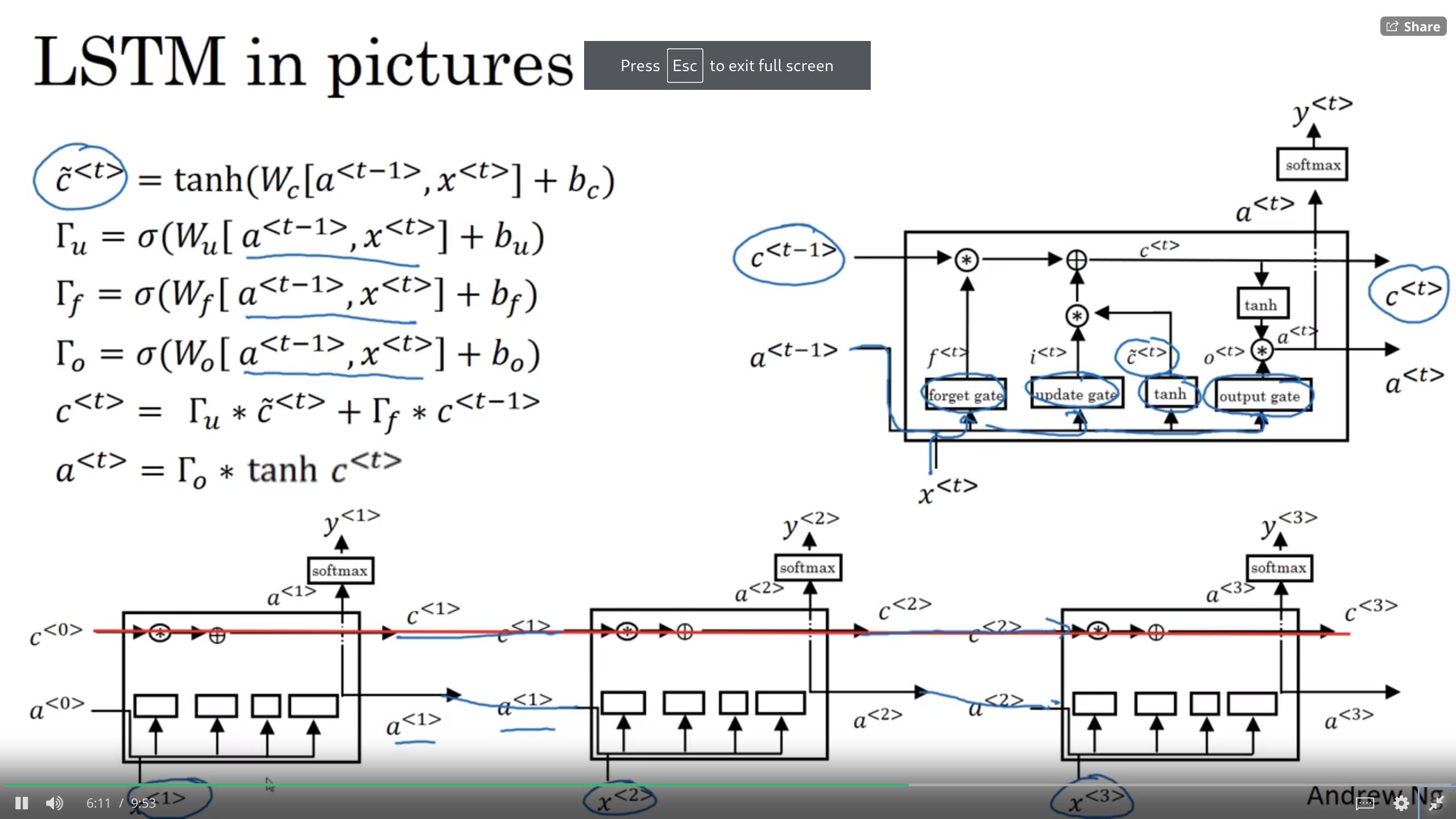
15.13. lstm
     even more powerful, general GRU
     GRU:
     C~<t> = tanh(Wc[ *Γ_r* ∗C<t-1>, x<t>] + b_c)
     Γ_u = sigmoid(W_u[C<t-1>, x<t>] + b_u)
     Γ_r = sigmoid(W_r[C<t-1>, x<t>] + b_r)
     C<t> = Γ_u∗C~<t> + (1−Γ_u)∗C<t−1>
     a<t> = c<t>
     LSTM:
     C~<t> = tanh(W_c[a<t-1>, x<t>] + b_c)
     Γ_u = sigmoid(W_u[a<t-1>, x<t>] + b_u)  (u - update)
     Γ_f = sigmoid(W_f[a<t-1>, x<t>] + b_f)  (f - forget)
     Γ_o = sigmoid(W_o[a<t-1>, x<t>] + b_o)  (o - output)
     C<t> = Γ_u * C~<t> + Γ_f * C<t−1>    (element-wise mult)
     a<t> = Γ_o * tanh(C<t)>
<lstm units diagram>
some variation – peephole connection (in Γ add after x<t> C<t-1> )
15.14. bidirectional rnns
He said, "Teddy ears are on sale!"
He said, "Teddy Roosevelt was a great President!"
can't fix with regular RNN/GRU/LSTM units - they are unidirectional
With BRNN:
you add one more a_backward unit along with a_forward
and connect it the same way to upper y, and lower x, but backwards horizontally (a<2> -> a<1>)
y_hat<1> ^ ^ | \ +—-+ +————-+ |a<1>| |a<1>_backward| +—-+ +————-+ ^ ^ | / x<1> y_hat
15.15. deep rnns
just introduce layers [l]
y_hat<1> …. ^ | +——-+ a[2]<0> –> |a[2]<1>| …. +——-+ ^ | +——-+ a[1]<0> –> |a[1]<1>| …. +——-+ ^ | x<1> a[2]<3> = g(Wa[2] ( a[2]<2>,a[1]<3> ) + b_a[2])
for rnns having 3 layers is already a lot
sometimes there are rnn layers just stacked (have vertical connection but no horizontal)
often this rectangular blocks are not just rnn but GRU/LSTM/BRNN
16. nlp
16.1. word representation
     V=[a,aaron,...,UNK]   10000
     1-hot representation

     Man(5391)      Woman(9853)
     [0]             ..
     [0]
     ..
     ..
     [1]
     ..
     [0]

     this vector is represented as O_5391

     one problem with this word representation is that it treats words separately, on itself, can't build relations to other words
     e.g. /orange juice/ and /apple juice/
     in other words there is no way to measure distance between words

     what if we can add some more features to each word
| man | woman | king | |
| gender | -1 | ||
| royal | 0.01 | ||
| age | 0.03 | ||
| food | 0.04 | ||
| … |
     e.g. we built 300 features *(embeddings*, cause word gets embedded into 300d space)
     we can use notation
     e_5391 - 300 dimensional vector
     in this case orange and apple are quite similar

     visualizing word embeddings 300d->2d
     t-SNE
     allows to see similar words close together
16.2. using word embeddings, transfer learning
     named entity recognition:
     sally johnson is an orange farmer
     robert lin is an apple farmer
                      durian cultivator    (if you have small set it's hard to recognize similarity)
     1. learn word embedding from large text corpus you can use big corpus of data 1b-100b words
     2. transfer embedding to new task with smaller training set. (100k words)
        now you can use smaller embedding vector e.g. 300 instead of 10000
     3. Optional: Continue to finetune the word embeddings with new data

     word embeddings make big difference when you have small training set so you can do transfer
     less useful for lang modeling, machine translation

     it has interesting relation to siamese face encoding (embedding)
       face -...-> 128d vector
16.3. properties of word embeddings
     analogies
     having 4 features (embeddings) <see embeddings table above>
     Man -> Women as King -> ?  (queen)
     e_5391 or e_man

     e_man - e_woman ~ [-2 0 0 0].T
     e_king - e_queen ~ [-2 0 0 0].T
     so thats is an idea - searching similarity
     if visualize in 300d - these are vectors (man->woman), and you look for parallel vectors (parallelogram)
       find word w: arg max(w) similarity(e_w, e_king - e_man + e_woman)
       you can get 30-75% analogy accuracy
     common similarity function - cosine
     sim(u,v)=u.T*v/(l2(u)*l2(v))
     or euqlidean distanc ||u-b||^2
     examples:
     ottawa:canada as nairobi:kenya
     big:bigger as tall:taller
16.4. embedding matrix
     vocab: a aaron orange.. zulu..unk
     we need to learn 300x10000 matrix
     orange - O_6257 - (one-hot embedding)
     Lets *E* - is this embeddings matrix
     E*O_6257 = (300;1) - embedding
     E*O_j = e_j
     in practice use specialized function just to get column ranger then multiply
16.5. how to learn word embeddings?
     lets say you building lang model
     /I    want     a     glass    of      orange ___/
     4343 9665     1     3852    6163     6257
      I     O_4343 -> E -> e4343
      want  O_...                \
      a     O_1 .....      e9665  ---->  feed into neural net -> softmax(10000)
      ...                        /           w[1],b[1]            w[2],b[2]

     input (eXXXX) - is 1800 (6x300 stacking) dimenstional vector
     you can decide to look only on previous 4 words (historical window)
     So this is a model with params you can learn: *E,w[1],b[1],w[2],b[2]*

     other context/target pairs
     you can pick context - 4 words on left and 4 words on the right
     I want   /a glass of orange __ to go along with/    my cereal
     It turns out you can use much simpler - just 1 last word or just 1 nearby word
     if you build a lang model - 4 is good, if just word embeddings - 1 is really good
16.6. word2vec
     /I want a glass of orange juice to go along with my cereal/
     How pick context/target?
     Lets pick orange and pick target randomly with some max distance
     orange,juice
     range,glass
     orange,my

     word2vec skip-gram model:
      Vocab 10000
      we want to learn this mapping:
      Context C("orange") -> Target t ("juice")     (or "my")
                 x  ---------------------------------->  y

                e_c=E*O_c
      O_c -> E -> e_c -> softmax -> y_hat

      Softmax
       probability of different target word given context
       P(t|c) = e^(Theta_t.T*e_c)/Sum(j=1:10000)(e^Theta_t.T*e_c)
       Theta_t = parameter associated with output t
       a chance of particular
      Loss
      L(y_hat,y)=-Sum(i=1:10000)(y_i*log(y_hat_i))    (negative log-likelyhood)
      y - one-hot vector  [00...1...0] (at 4834)
      params to learn here: *E Theta_t*
      computationally not very good - a Sum over entire vocab
      but you can optimize with hierarchical softmax (basically binary tree splitting vocab)

     how to sample context c?
     uniformly random - but then you get too much the/of/a/and/...
     P(c) - in practice there are different heuristics to balance this out
16.7. negative sampling
     learning problem:
     pick 1 positive and sample some negative (just randomly pick from voc) examples of length k
     for smaller datasets k=5-20, for larger l=2-5
     k+1

        x                 y
     (c)ontext+word(t)   target?(y)
     orange   +juice      1
     orange   +king       0
     ...

     define logistic regression model
     P(y=1|c,t) = sigmoid(Theta_t.T*e_c)

     for a given context
     orange(6257)

     O_6257 -> E -> e_6257 ->...10k logistic regression problems - one of them will be predicting juice, another king

     on each learning iteration
     we pick only 5 (1+4 random) and train (not all 10000)
     it is relatively cheap to train k+1 logistic units

     how to choose negative?
     you can sample based on distribution in your corpus, but then again the/of/a/..
     uniformely - again not representative
     Miklov(author) - came up with empirical formula:
       f(w_i) - frequency of word in english text
     P(w_i) = f(w_i)/Sum10000(f(w_j)^(3/4))
16.8. GloVe algorithm
     simplicity
     previously we picked c,t
     lets say x_ij = #times j appears in context of i
     i=c
     j=t
     Model:
     minimize   Sum(i,j=1:10000) f(x_ij) (Theta_i.T*e_j + b_i + b_j' - log(x_ij))^2
     weighting term - f(x_ij) - if x_ij=0 then f=0,  and gives some computation to 'durion'
     Theta_i, e_i - are symmetric (play same role)
     so after training you can apply some averaging
     e_w_final = (e_w + Theta_w)/2

     the model is simple but it really works

     a note on featurization view of word embeddings
     putting vectors e_w1 e_w2 on axis and using some linear algebra transformations we can show
     Theta_i.T*e_j = (A*Theta_i).T*(A.T*e_j)=Theta_i.T +A.T*A.-T+ e_j
     we may learn some very complex features but in linear space we can transform them back to proper features (gender,royal,age,etc)
16.9. sentiment classification
     with embeddings you can build this model even with small dataset
     The dessert is excellent
     simple way - just avg all embeddings of the words in sentence and pipe into softmax (output 1-5 rating)

     rnn for sentiment classification - this works much better
     many to one
                                                        y_hat
                                                        softmax
a<0> -> a<1>    ->    a<2>     a<3>     a<4>            a<10>
        e1852         e4966    e4427    e3882           e330
        E             E        E        E               E
     Completely    lacking     in     good   .....   ambience
16.10. problem of bias in word embeddings
     man:computer_programmer as woman:homemaker
     gender,ethnicity,age,sexual orientation
     lets say we already learned embeddings
     1. identify bias direction
        e_he-e_she, e_male-e_female .. -> do average - this will identify bias vector direction
     2. neutralization. For every word that is not definitial, project to get rid of bias
        project the word on non-bias direction (like axis)
        how do you decide which words neutraliza - train a linear classifier
     3. equalize pairs. grandmother/grandfather - move them so they are on both directions of non-bias and on the same distance
        this makes them on the same distance from e.g. babysitter
17. sequence to sequence models
17.1. basic models
     e.g. translate from french to english
     encoder-decoder network
     in decoder do the sequencing piping output as input

     the same principle for image captioning
     take AlexNet and then pipe into generating rnn - synthesize caption
17.2. pick the most likely sentence
     lets take language model - can learn probability of sentence

     machine translation - very similar but
     starts with encoder (conditional language model)
     output P(y<1>,...|x) - when outputting how to sample not on random but the best english translation?
     you can do greedy search - pick word-by-word based on word-most-likely
17.3. beam search (TODO)
     step1
     param B=3 (beam width)
     at first unit of decoder
     P(y<1>|x)
     step2
17.4. bleu score (TODO)
17.5. attention model (TODO)
18. speech recognition - audio data
18.1. speech recognition (TODO)
audio clip -> transcript